Histograms, Scatter Plots and Subplots

Line and bar charts summarise. Histograms and scatter plots show every data point, which is how you discover what the averages hide: two groups of students, an outlier, a relationship between two numbers.

Histograms: how are values spread?#

A histogram splits numbers into ranges (bins) and counts how many fall in each:

import numpy as np
import matplotlib.pyplot as plt

rng = np.random.default_rng(1)
marks = np.clip(rng.normal(68, 12, 300), 0, 100)

fig, ax = plt.subplots(figsize=(7, 4))
ax.hist(marks, bins=15, color="#0a7d4f", edgecolor="white")
ax.axvline(marks.mean(), color="tab:red", linestyle="--", label=f"mean = {marks.mean():.1f}")
ax.set_title("Most students scored between 55 and 80")
ax.set_xlabel("Marks")
ax.set_ylabel("Number of students")
ax.legend()
plt.show()

rng.normal(68, 12, 300) generates 300 realistic marks around 68. axvline draws a vertical line at the mean.

Scatter plots: are two numbers related?#

Each dot is one row: x is one column, y is another.

import numpy as np
import matplotlib.pyplot as plt

rng = np.random.default_rng(7)
hours = rng.uniform(0, 10, 60)
score = 35 + 5.5 * hours + rng.normal(0, 7, 60)

fig, ax = plt.subplots(figsize=(7, 4))
ax.scatter(hours, score, alpha=0.7)
ax.set_title("More study hours, higher scores")
ax.set_xlabel("Hours studied per week")
ax.set_ylabel("Test score")
plt.show()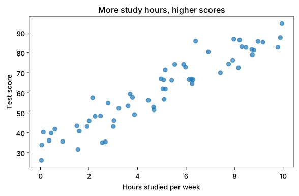

The dots go up from left to right: a positive relationship. alpha=0.7 makes dots slightly see-through, so overlapping points are visible. In the Machine Learning course you’ll fit a line through exactly this kind of data.

Careful

A relationship isn’t proof that one thing causes the other. Ice-cream sales and drowning both rise in summer; neither causes the other.

Subplots: several charts in one figure#

plt.subplots(rows, cols) returns a grid of axes. Draw each chart on its own ax:

import numpy as np
import matplotlib.pyplot as plt

months = ["Jan", "Feb", "Mar", "Apr", "May", "Jun"]
revenue = [42, 45, 39, 51, 58, 63]
orders = [310, 330, 290, 360, 400, 455]

fig, (ax1, ax2) = plt.subplots(1, 2, figsize=(10, 3.8))
ax1.plot(months, revenue, marker="o", color="tab:green")
ax1.set_title("Revenue (₹ lakh)")
ax2.bar(months, orders, color="tab:blue")
ax2.set_title("Orders")
fig.suptitle("First half of the year", fontweight="bold")
fig.tight_layout()
plt.show()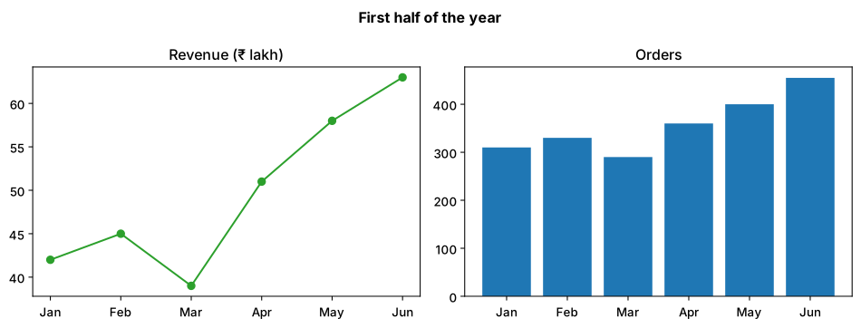

• plt.subplots(1, 2): 1 row, 2 columns.
• fig.suptitle(): one title over the whole figure.
• fig.tight_layout(): stops labels from overlapping.

Summary#

• ax.hist(values, bins=...) shows the spread of one column.
• ax.scatter(x, y) shows whether two columns move together.
• plt.subplots(r, c) gives a grid of axes for side-by-side comparisons.