Relationships and Heatmaps with Seaborn

Before building a machine learning model, data scientists look for relationships: which columns rise and fall together? Seaborn makes that exploration fast. This lesson covers scatter plots with a trend line and the correlation heatmap, a chart you’ll see in almost every data science notebook.

import numpy as np
import pandas as pd
import seaborn as sns
import matplotlib.pyplot as plt

rng = np.random.default_rng(11)
n = 150
area = rng.uniform(500, 2500, n)
rooms = np.clip((area / 550 + rng.normal(0, 0.7, n)).round(), 1, 6)
age = rng.uniform(0, 30, n).round()
price = (2500000 + area * 5200 + rooms * 150000 - age * 150000 + rng.normal(0, 600000, n)) / 100000
homes = pd.DataFrame({"area_sqft": area.round(), "rooms": rooms, "age_years": age, "price_lakh": price.round(1)})
sns.set_theme(style="whitegrid")
print(homes.describe().round(1).loc[["mean", "min", "max"]])

Output:

      area_sqft  rooms  age_years  price_lakh
mean     1409.0    2.6       14.8        79.9
min       534.0    1.0        0.0        16.6
max      2498.0    6.0       29.0       167.3

A made-up but realistic table of 150 homes: area, rooms, age and price.

scatterplot with hue#

fig, ax = plt.subplots(figsize=(7, 4))
sns.scatterplot(data=homes, x="area_sqft", y="price_lakh", hue="rooms", palette="viridis", ax=ax)
ax.set_title("Bigger homes cost more")
plt.show()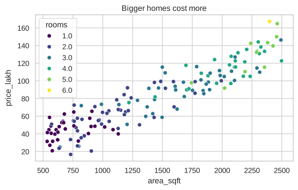

Colour (hue) adds a third column to a 2-D chart: you can see bigger homes also tend to have more rooms.

regplot: add the trend line#

fig, ax = plt.subplots(figsize=(7, 4))
sns.regplot(data=homes, x="age_years", y="price_lakh", scatter_kws={"alpha": 0.5}, line_kws={"color": "tab:red"}, ax=ax)
ax.set_title("Older homes are a little cheaper")
plt.show()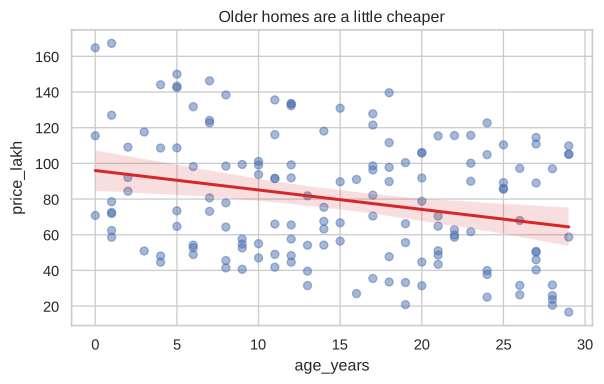

regplot fits a straight line through the points (a linear regression, which you’ll build yourself in the Machine Learning course). The shaded band shows the uncertainty.

Correlation heatmap#

Correlation is a number from -1 to 1 that measures how strongly two columns move together:

• close to 1: when one rises, the other rises;
• close to -1: when one rises, the other falls;
• close to 0: no straight-line relationship.

corr = homes.corr().round(2)
print(corr["price_lakh"])

Output:

area_sqft     0.92
rooms         0.81
age_years    -0.26
price_lakh    1.00
Name: price_lakh, dtype: float64

A heatmap shows the whole table as colours:

fig, ax = plt.subplots(figsize=(6, 4.5))
sns.heatmap(corr, annot=True, cmap="RdYlGn", vmin=-1, vmax=1, ax=ax)
ax.set_title("Which columns move together?")
plt.show()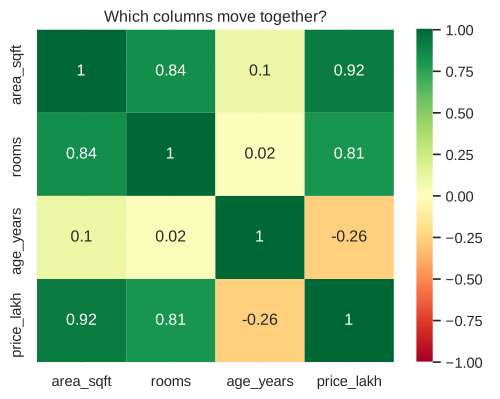

Area has the strongest link to price (0.92), and age a weak negative one (-0.26), so it would be the most useful input for a model predicting prices.

Mini dashboard#

Combine what you’ve learned into one figure you could put in a report:

fig, axes = plt.subplots(1, 3, figsize=(13, 3.8))
sns.histplot(homes["price_lakh"], bins=20, ax=axes[0])
axes[0].set_title("Price distribution")
sns.boxplot(data=homes, x="rooms", y="price_lakh", ax=axes[1])
axes[1].set_title("Price by rooms")
sns.regplot(data=homes, x="area_sqft", y="price_lakh", scatter_kws={"s": 12}, ax=axes[2])
axes[2].set_title("Price vs area")
fig.suptitle("Home prices at a glance", fontweight="bold")
fig.tight_layout()
plt.show()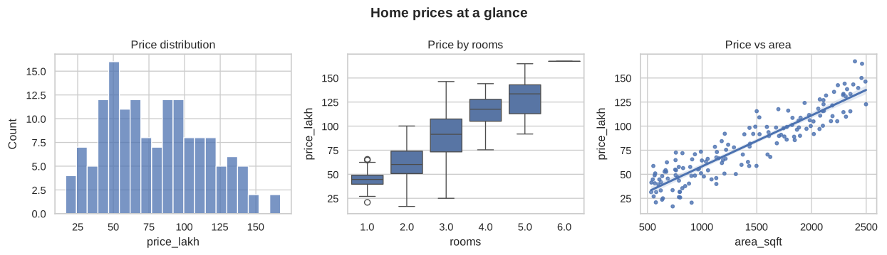

Next step

You’ve explored the data and found that area predicts price well. In the Machine Learning course, you’ll train a model that actually makes that prediction.

Summary#

• sns.scatterplot(..., hue=...) shows a relationship plus a category.
• sns.regplot adds a trend line.
• df.corr() + sns.heatmap(annot=True) shows which columns move together.
• Combine charts with plt.subplots for a simple dashboard.