Seaborn Basics

Seaborn sits on top of Matplotlib and speaks Pandas. You hand it a DataFrame and column names, and it does the grouping, averaging and colouring for you. Charts that take ten lines in Matplotlib take one.

pip install seaborn

We’ll use this small dataset of students:

import numpy as np
import pandas as pd
import seaborn as sns
import matplotlib.pyplot as plt

rng = np.random.default_rng(3)
n = 120
df = pd.DataFrame({
    "course": rng.choice(["Python", "Java", "Web"], n, p=[0.45, 0.3, 0.25]),
    "gender": rng.choice(["Female", "Male"], n),
    "hours": rng.uniform(1, 12, n).round(1),
})
df["score"] = (40 + 4.5 * df["hours"] + rng.normal(0, 8, n)).clip(0, 100).round()
sns.set_theme(style="whitegrid")
print(df.head())

Output:

   course  gender  hours  score
0  Python  Female    6.7   66.0
1  Python    Male    2.8   67.0
2     Web  Female    5.9   59.0
3    Java    Male   10.6  100.0
4  Python    Male    7.2   72.0

sns.set_theme() switches on Seaborn’s clean default look for every chart after it.

countplot: how many in each category?#

fig, ax = plt.subplots(figsize=(7, 4))
sns.countplot(data=df, x="course", order=df["course"].value_counts().index, ax=ax)
ax.set_title("Python is our most chosen course")
plt.show()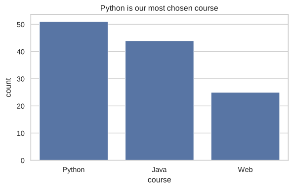

No value_counts, no loop: Seaborn counted the rows itself.

barplot: average per category#

fig, ax = plt.subplots(figsize=(7, 4))
sns.barplot(data=df, x="course", y="score", hue="gender", ax=ax)
ax.set_title("Average score by course and gender")
plt.show()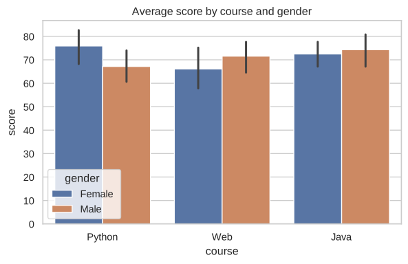

barplot shows the mean of y for each x, and hue splits each bar by a second category. The small black lines are error bars: how sure we are about each average. Long lines mean few students or very mixed scores.

histplot: distribution, optionally by group#

fig, ax = plt.subplots(figsize=(7, 4))
sns.histplot(data=df, x="score", hue="course", kde=True, element="step", ax=ax)
ax.set_title("Score distribution per course")
plt.show()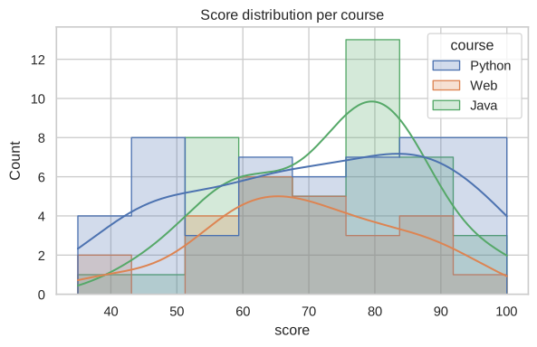

kde=True adds a smooth curve that estimates the shape, which is easier to compare than bars.

boxplot: spread and outliers at a glance#

fig, ax = plt.subplots(figsize=(7, 4))
sns.boxplot(data=df, x="course", y="hours", ax=ax)
ax.set_title("Weekly study hours per course")
plt.show()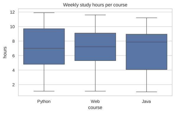

How to read a box:

• The line in the middle is the median.
• The box covers the middle 50% of students (from the 25th to the 75th percentile).
• The whiskers reach the rest of the normal range; dots beyond them are outliers.

Quick check

Seaborn functions take data=df and column names as strings: x="course", not x=df["course"]. Both work, but the first gives automatic axis labels.

Summary#

Question	Seaborn
How many per category?	sns.countplot
Average per category?	sns.barplot
How are values spread?	sns.histplot, sns.boxplot
Split by another category	add hue="column"